Risk Management in Investment Portfolios: Strategies for Mitigating Volatility

The number worth opening any investment risk management discussion with in 2026 is not the S&P 500 level. It is the VIX, which spent the 12 months from May 2025 to May 2026 in a 13.38-to-35.30 range, surged above 30 in March 2026 on tariff and geopolitical concerns, and fell back below 20 by mid-April. What that measures is the market's pricing of expected 30-day S&P volatility — implied, not realized — which is a more useful signal than spot returns because it reveals what option-market participants are paying to hedge against the next month. What it does not tell you is the path: a VIX of 20 can stay at 20 for months, or it can spike to 40 in two trading sessions. The point of risk management is to build a portfolio whose performance does not depend on guessing which.

The rest of this article is the disciplined toolkit. Risk metrics with the formulas and thresholds the typical retail explainer skips. Named portfolio templates (60/40, All-Weather, three-fund) with concrete drawdowns from 2008, 2020, and 2022. The hedging menu — cash buffer, stop-losses, protective puts, collars, tail-risk ETFs, buffer ETFs — with an honest cost-benefit on each. And the rebalancing rule that actually works in the data, not the calendar rule the brokerage marketing copy defaults to.

The 2026 Volatility Regime Snapshot

Three numbers anchor the May 2026 risk-management conversation:

Indicator	Reading
VIX 12-month range (May 2025–May 2026)	13.38 to 35.30
S&P 500 YTD through early April 2026	-4%, after +18% in 2025
S&P 500 forward P/E	20.9 (April 2026)

What this snapshot does not tell you is the regime underneath the numbers. A forward P/E of 20.9 against a 10-year historical median in the 16–18 range means the market is pricing meaningful earnings growth from current levels; that growth assumption is itself a risk factor that does not show up in the VIX. The honest read for an allocator is that the headline volatility metric is mid-range and rising, but the valuation backdrop carries embedded downside that volatility alone does not capture. Risk management in this regime is more about position sizing and rebalancing discipline than about hedging the next 30-day move.

What Kinds of Risk a Portfolio Actually Faces

The vocabulary every retail explainer uses splits portfolio risk into systematic and unsystematic, and that split is correct but incomplete. The disciplined breakdown that matters for decision-making:

• Market (systematic) risk: the risk that the broad market drops. Cannot be diversified away within an asset class; can be partially offset by holding non-correlated asset classes.
• Idiosyncratic (unsystematic) risk: the risk of a single position blowing up. Diversifiable — the case for owning ETFs rather than concentrated stocks.
• Inflation risk: the risk that real returns fall short of nominal even when nominal returns look fine. The 2022 inflation episode was textbook — bond and equity returns were both negative in nominal terms and far worse in real terms.
• Interest-rate risk: bond duration matters most when rates move. A 10-year Treasury position drops ~7% when 10-year yields rise 100 basis points; a 2-year position drops ~2%.
• Liquidity risk: the risk that you cannot exit at quoted prices. Mostly invisible until it matters, then matters a lot — the March 2020 ETF discount to NAV episode is the case study.
• Credit risk: the risk that a fixed-income issuer defaults or downgrades. Concentrated in high-yield and emerging-market debt; mostly absent from Treasury exposure.
• Correlation risk: the risk that the diversification you assumed disappears when you need it. This is the 2022 60/40 problem — when both stocks and bonds drop together, the textbook risk-reduction story stops working.

Most retail portfolios are managed against the first two and ignore the rest. The 2022 experience exposed that asymmetry; the toolkit below assumes you actually care about all seven.

Risk Metrics Cheat Sheet

The four risk metrics worth knowing, with their formulas and the rule-of-thumb thresholds that most explainers skip.

Metric	Formula	What it measures	Good / OK / Concerning
Sharpe ratio	(Portfolio return − risk-free rate) / Portfolio standard deviation	Total-volatility-adjusted excess return	>2 very good; >1 acceptable; <0.5 concerning
Sortino ratio	(Portfolio return − risk-free rate) / Downside deviation	Like Sharpe, but penalizes only downside volatility	Higher than Sharpe for the same portfolio; >1.5 acceptable; >2 strong
Treynor ratio	(Portfolio return − risk-free rate) / Portfolio beta	Beta-adjusted excess return (systematic risk only)	Use to compare diversified portfolios; >0.10 is generally acceptable
Value at Risk (VaR)	Statistical estimate of maximum expected loss at a given confidence level over a given period	1-day 95% VaR on $100k S&P 500 ≈ $2,000–$3,000 in normal vol regimes	Compare VaR across portfolios; the metric only matters relative to your loss tolerance
Maximum drawdown	Largest peak-to-trough drop over a measurement period	The worst-case experience an investor would have lived through	Lower is better — and this is the metric retirees should weight most heavily

Sharpe vs Sortino: When the Distinction Matters

The Sharpe ratio penalizes all volatility — upside and downside. That is statistically clean but practically unhelpful for any strategy whose upside is asymmetric. A long-only equity position whose annualized return includes a few +10% months gets penalized by Sharpe for the same reason it gets penalized for -10% months. Sortino fixes that by computing the denominator using only periods of negative return.

Practical rule: for a long-only diversified equity or balanced portfolio, Sharpe is the standard reference metric and most reported risk-adjusted returns use it. For asymmetric strategies (covered-call income, options selling, long-vol hedges), Sortino is the more honest metric and the one to ask about explicitly. A fund that reports a great Sharpe but does not report Sortino is doing it deliberately, usually because the Sortino is significantly worse.

Value at Risk and Why Retirees Care Most About Max Drawdown

VaR answers "how much can I lose in a normal bad period." A 1-day 95% VaR of $3,000 on a $100k portfolio means: in 95% of one-day windows, your loss will be smaller than $3,000. What VaR does not answer is what happens in the 5% tail — the financial-crisis windows. The 2008 max drawdown for the S&P 500 was 55% peak-to-trough; the 2020 pandemic max drawdown was 34%; the 2022 60/40 max drawdown was 17.5%. None of those would have shown up cleanly in a VaR estimate built from prior-period data.

For investors in accumulation phase, max drawdown is uncomfortable but survivable — share prices recover, share counts grow on contributions, dividend reinvestment compounds. For retirees actively drawing down a portfolio, max drawdown is the single most important risk metric. Selling at the bottom to fund living expenses is the mechanism that converts a temporary drawdown into a permanent loss, and the only defense is allocating before retirement to a portfolio whose drawdown profile you can actually live through.

Named Portfolio Templates

The retail risk-management discussion is often pitched abstractly — "diversify," "balance" — when the more useful question is which of a few concrete portfolio templates matches your situation and what its measured drawdown history actually is. Three templates cover most of the practical decision space.

100% US Equities (S&P 500 / VTI). Maximum long-run expected return for a US-investor portfolio; maximum drawdown exposure. Historical drawdowns: -55% in 2008, -34% in March 2020. The right answer for accumulation-phase investors with 10+ year horizons; the wrong answer for anyone who would sell at the bottom.

60/40 Portfolio. 60% US equities, 40% bonds (a mix of intermediate Treasuries and aggregate). The historical retail default. 2022 was -17.5%, the worst year since 1937, fourth-worst in 200 years. It then recovered: +17.2% in 2023, ~15% in 2024, ~15% in 2025, and +3.89% YTD through April 25, 2026. The 60/40 round-trip is the most important risk-management story of the last four years.

All-Weather Portfolio. Ray Dalio's allocation, designed to perform across all four economic regimes (growth and inflation each up or down). The published allocation: 30% US equities (VTI), 40% long-term Treasuries (TLT), 15% intermediate Treasuries (IEF), 7.5% gold (GLD), 7.5% commodities (DBC). 26-year CAGR (1999–2025) approximately 4.65% — lower than 60/40, but with materially smaller drawdowns. State Street and Bridgewater launched the SPDR Bridgewater All Weather ETF (ALLW) in March 2025, making the strategy available as a single-ticker holding.

Template	Allocation	Mechanism	Best for	Trade-off
100% Equities (VTI)	100% broad US equities	Maximum equity-risk premium capture	Long-horizon accumulation, high risk tolerance	Largest drawdowns; behavioral risk of selling at bottoms
60/40	60% equities, 40% bonds	Equity returns with bond ballast	Balanced accumulation; pre-retirement	Failed in 2022 inflation shock; recovered in 2023–25
All-Weather	30/40/15/7.5/7.5	Designed for regime diversification	Risk-averse investors; near-retirement	Lower long-run CAGR (~4.65%) than 60/40
Three-Fund	VTI / VXUS / BND in chosen ratio	Maximum simplicity + diversification	Hands-off retail; "set and rebalance"	Adds international currency risk; rebalancing inertia

Is 60/40 Dead? The 2022 to 2026 Round-Trip

The "60/40 is dead" thesis was loud in late 2022 and early 2023 after the worst drawdown for the strategy in nearly a century. The math underneath the thesis was a single observation: stock-bond correlation went sharply positive during the 2022 inflation shock, and a portfolio whose risk reduction depends on negative or low correlation stops working when correlation flips.

Three years later, the data has reset. The 12-month rolling stock-bond correlation peaked at 0.80 mid-2024 and fell to 0.16 by late 2025, restoring the diversification benefit that broke down in 2022. The 36-month correlation eased from a December 2024 peak of 0.66 to 0.48 by September 2025. 60/40's 2023–2025 cumulative return is competitive with most institutional benchmarks. The strategy is not dead; the 2022 episode was a regime-specific failure during an inflation shock that has substantially moderated.

The honest caveat — the one nobody marketing 60/40 talks about — is that the correlation reset is contingent on inflation moderating. The IMF flagged in February 2026 that "bonds are increasingly moving in tandem with stocks" during inflation-regime shocks, making 60/40 and risk parity more vulnerable in environments where inflation expectations stay elevated. With inflation expected to hold above 3% through 2026, the 2022 vulnerability remains a latent feature of the portfolio. The disciplined answer is to allocate to 60/40 with the explicit acknowledgement that the diversification benefit weakens precisely when inflation reasserts — and to size the equity sleeve such that the portfolio survives a recurrence.

Drawdown Comparison: 100% S&P vs 60/40 vs All-Weather

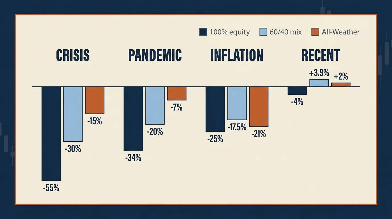
The single piece of data that converts the abstract template discussion into actionable risk allocation is a side-by-side drawdown comparison across the recent stress periods. Approximate peak-to-trough drawdowns:

Period	100% S&P 500	60/40	All-Weather
2008 (Financial Crisis)	-55%	~-30%	~-15% (gold partially offset)
2020 (COVID, Feb–Mar)	-34%	~-20%	~-7% (Treasuries rallied)
2022 (inflation shock)	-25% (cal year)	-17.5%	~-21% (worst-ever year for All-Weather; bonds + gold + commodities all down)
2026 YTD through early April	-4%	+3.89%	~+2%

The pattern is what matters. All-Weather wins the 2008 and 2020 drawdown comparisons by a wide margin because the Treasury allocation provides genuine diversification when equities fall. 60/40 wins the 2026 comparison because growth-and-inflation moderation favors the conventional asset-class mix. The 2022 inflation episode broke both diversified templates for the same reason — when bonds, gold, and commodities all sell off simultaneously with equities, no traditional correlation-based hedge works.

The honest implication: there is no template that wins every regime. The disciplined choice is the one whose worst regime you can actually live through, not the one whose best regime sounds best on paper.

Loading image...

Stop-Loss Orders: Market, Limit, Trailing

Stop-loss orders are the most misunderstood retail risk tool. The vocabulary distinguishes three structurally different instruments.

Market stop. Triggers a market sell when the price hits a specified level. The execution price is whatever the market clears at — which in a gap-down or fast market can be materially below the trigger. Useful for low-volatility positions; dangerous for thin-volume or earnings-driven names.

Limit stop. Triggers a sell at or above a specified limit price. Protects against bad execution but may not execute at all if the price gaps below the limit. The opposite trade-off from a market stop.

Trailing stop. Follows the position's high-water mark by a percentage or dollar amount. The most useful retail variant. Worked example: a $10,000 position in an ETF with an 8% trailing stop. As the position rises from $10,000 to $12,000, the stop trails up to $11,040 (8% below $12,000). If the position then falls to $11,040, the stop triggers; you have locked in $1,040 of the unrealized gain instead of riding it back down.

The two structural limitations of stop-loss orders that retail explainers consistently undersell:

1. They protect against drawdown, not against being wrong. A stop-loss exits a position that has fallen below your tolerance threshold; it does not tell you whether the position should have been entered in the first place. The fix is sizing and selection, not stop-loss tactics.
2. They are vulnerable to whipsaws. A position that drops to your stop, triggers, and then immediately reverses leaves you out at the worst possible price. Stops sized too tightly relative to the underlying volatility get whipsawed routinely. The 8% trailing stop in the worked example above is appropriate for a low-volatility ETF; a high-volatility single stock might need 15–20% for the same protective intent.

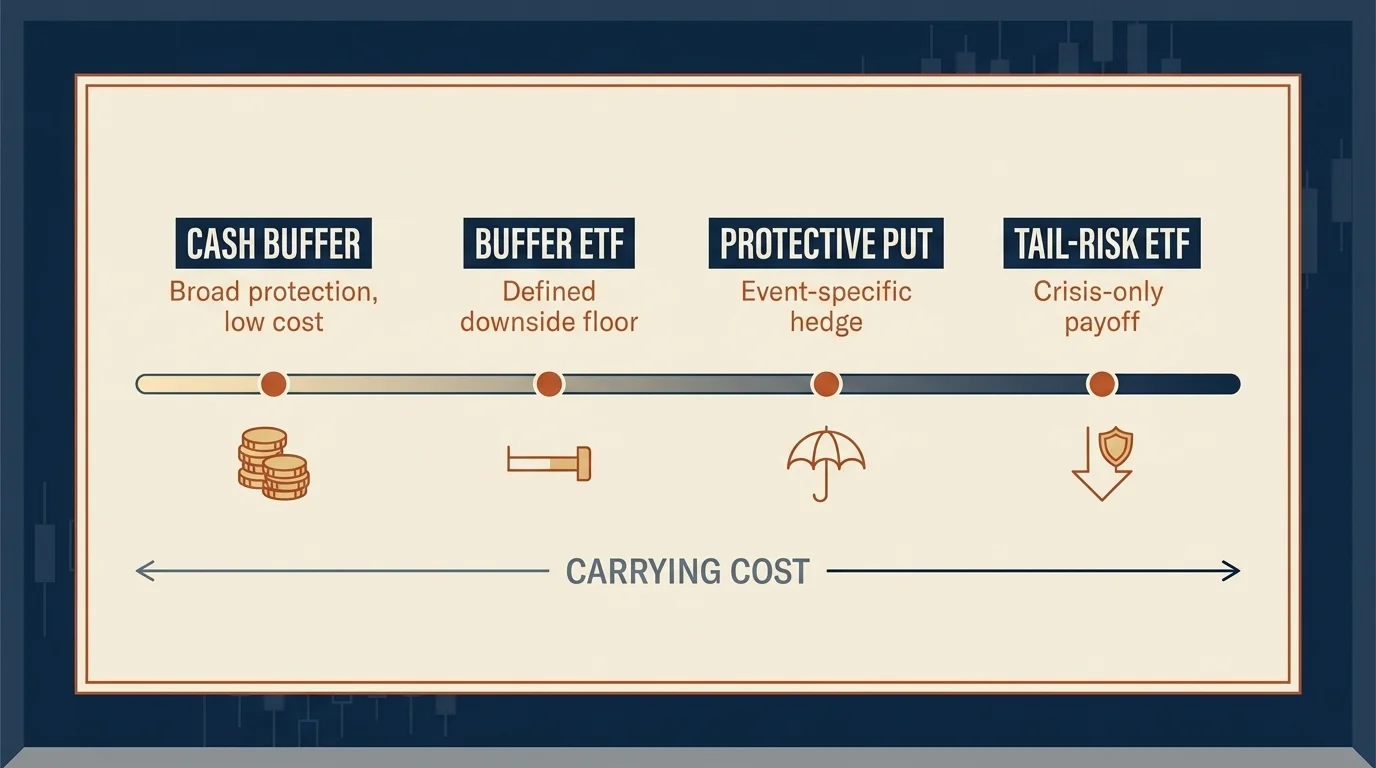
Modern Hedging Toolkit

The retail hedging menu has expanded substantially since 2022. The comparison below shows the practical options, their cost structures, and when each fits.

Hedge	What it does	Cost	Best for	Honest limitation
Cash / short-Treasury buffer	Holds 5–15% of portfolio in cash or T-bills	Opportunity cost (foregone equity return)	Every retail portfolio	Returns near short rate; not a directional hedge
Protective puts	Buy put option below current price	Premium decays over time	Specific event hedges (earnings, macro)	Premium drag during quiet markets
Collar (zero-cost or near)	Buy put + sell call at higher strike	Often near-zero net premium	Concentrated equity positions you cannot sell	Caps upside; complex to maintain
Tail-risk ETFs (TAIL, CAOS)	Hold deep OTM puts as portfolio insurance	CAOS 0.63% ER, $374M AUM; deep OTM at 30–60% below spot	Catastrophic-loss insurance	Bleeds during normal markets; TAIL gained ~16% in 2026 selloff but underperforms in quiet years
Managed-futures ETFs (DBMF)	Long/short trend-following across asset classes	DBMF 0.95%+ ER	Crisis-alpha sleeve; low equity correlation	DBMF earned Four-Star Morningstar rating as of March 2026; outperformed SocGen CTA Index by 700+ bps in 2025, but down 2.86% YTD through May 2025
Buffer ETFs	Capped upside / defined downside protection over a 12-month outcome period	Typically 0.75–0.85% ER	Pre-retirement allocations needing soft downside floor	$70B+ AUM category; 98% in buffer strategies; cap on upside reduces compounding
Covered-call ETFs (JEPI, JEPQ)	Sell calls to generate income	Implicit cost: capped upside	Income with partial downside cushion	Not a true hedge; reduces volatility but does not protect tail
Inverse ETFs (SH, SDS)	Negative beta exposure	Ongoing tracking decay	Short-duration tactical hedges	Compounding decay makes them inappropriate for buy-and-hold; intended for days, not years

Is Hedging Worth It for Retail?

The honest answer is "often no." The cost structure of most active hedges — option premium decay, tail-ETF carrying cost, buffer-ETF cap on upside — compounds against you during the typical-year majority when no significant drawdown occurs. The case for a hedge needs to clear two bars: the cost has to be tolerable relative to portfolio size, and the hedge has to actually pay off when you need it.

For the typical retail allocator, the most cost-effective "hedge" is the cash-and-short-Treasury buffer plus a disciplined allocation away from 100% equities. Five to fifteen percent of the portfolio in T-bills or a short-Treasury ETF (SGOV, BIL) earns near-the-short-rate while providing genuine dry powder during drawdowns. The compound annual cost is low — current short rates are competitive with most "safe" alternatives — and the protective behavior during a drawdown is high: you have cash to rebalance into equities when prices fall.

Active hedges (puts, collars, tail-risk ETFs, managed futures) make sense for specific situations: concentrated equity positions you cannot sell for tax reasons, defined event risk (a known earnings or macro catalyst), pre-retirement portfolios where one large drawdown changes retirement math, or institutional-style allocators with the operational sophistication to maintain them. They do not make sense as a default retail discipline.

Loading image...

Stress Testing: VaR and Monte Carlo Retirement

The two practical stress tests for a retail portfolio answer different questions.

Value at Risk answers: in a normal-volatility regime, what is the largest expected loss over a one-day window at a 95% confidence level? Useful for risk-budgeting (how big should this position be), less useful for tail planning.

Monte Carlo retirement simulation answers the question that actually matters for most allocators: given my contribution rate, allocation, and withdrawal plan, what is the probability that my portfolio survives the full retirement horizon? A well-designed Monte Carlo runs thousands of randomized return paths against the portfolio and reports failure rates. Target failure rate for a typical retiree: less than 10% over a 30-year horizon. A failure rate meaningfully above the target threshold means the plan needs adjusting — higher contributions, longer working horizon, lower withdrawal rate, or a more drawdown-resilient allocation.

Free Monte Carlo calculators are available from Vanguard, Schwab, and several independent fintech platforms. The methodology that matters: use rolling historical return distributions rather than assumed normal distributions, and run the simulation against your actual projected expense profile, not the abstract "4% rule." The 4% safe withdrawal rate works as a planning anchor; the Monte Carlo run reveals whether your specific situation supports it.

How Often to Rebalance: The Vanguard 200 bps Rule

The brokerage marketing default is "rebalance annually." That answer is correct only by accident. Vanguard's December 2024 research found that for target-date funds, a 200 basis point threshold with a 175 basis point destination minimizes transaction cost relative to monthly rebalancing. Translated for retail 60/40 portfolios: a 5% absolute drift band with annual or semi-annual monitoring balances risk control and transaction cost.

The practical implementation: set target allocation (60/40, three-fund, or whatever template you chose). Review the actual allocation every six months. If any asset class has drifted more than 5 percentage points from target, rebalance back. If not, do nothing. The discipline is in not trading absent the threshold trigger — most over-rebalancing comes from monitoring monthly and trading on noise.

For taxable accounts, two refinements: rebalance using new contributions first (buy more of what is underweight) before triggering a sale, and consider rebalancing into a tax-loss harvest event when one is available. The combination preserves the discipline while minimizing realized tax drag.

A Worked End-to-End Example: $100k Retail Portfolio

To make the abstract toolkit concrete, here is how the pieces fit together for a hypothetical $100,000 retail portfolio with a 15-year horizon:

• Allocation: 60% in a US equity ETF (VTI), 30% in a bond ETF (BND), 10% in cash/short-Treasury (SGOV).
• Risk metrics: target Sharpe above 0.8 over rolling 3-year periods, max drawdown tolerance approximately 25%.
• Stop-loss policy: none on the core ETF positions (whipsaw cost outweighs benefit on diversified holdings); 8% trailing stop on any single-stock positions if added later.
• Hedging: cash buffer is the hedge. No tail-risk ETF unless portfolio size grows materially larger and concentrated positions are added.
• Rebalancing: review every six months. If allocation drifts more than 5 percentage points from target, rebalance back. New contributions go to whichever sleeve is underweight.
• Stress test: run a Monte Carlo annually against expected retirement-year withdrawals; target failure rate below 10%.

That portfolio does not optimize for the highest possible return. It optimizes for the highest return that the investor will actually hold through the inevitable drawdown. The behavioral discipline of being able to hold the position is the binding constraint, not the theoretical math.

What Would Change My View

The thesis underneath this article is that risk management for a retail portfolio comes down to three disciplines: a sensible allocation matched to your actual risk tolerance, a cash buffer that lets you survive drawdowns without selling at bottoms, and a mechanical rebalancing rule that takes emotion out of the decision. Active hedges (tail-risk ETFs, options, buffer products) are useful for specific situations and dilutive for most retail portfolios over multi-decade horizons.

What would change my view? One thing, specifically: a sustained correlation regime in which stock-bond correlation stays above 0.5 for multiple years while inflation also stays above 3%. That combination would mean the IMF's February 2026 caution about regime fragility had hardened into a structural feature, not a transient episode. In that world, the case for tail-risk hedges and managed-futures sleeves would strengthen substantially; the case for 60/40 would weaken; the case for All-Weather (which performed poorly in 2022 specifically because all of its non-equity sleeves fell together) would also weaken. The disciplined response would be a higher cash buffer, a larger short-duration Treasury allocation, and a small managed-futures sleeve. Until that data prints, the framework above looks like the right answer for the regime we actually have.

I am watching the 12-month stock-bond correlation, the realized inflation rate, and the VIX 6-month moving average — that combination, not any single number, is what would tell me the regime has changed.

---

This article is for educational purposes only and is not individual financial advice. Risk-management metrics, historical drawdowns, hedging strategies, and fund expense ratios change frequently. Past performance does not guarantee future returns; correlation regimes that held for decades can shift in months. Consult a licensed financial advisor for guidance matched to your specific situation and risk tolerance, and read each fund's prospectus before allocating capital.